Invertible NNs
可逆神经网络被提出,可帮助降低显存占用。当前层的结果可由当前层参数和下一层结果反推得到,从而只需要保存参数和最后一层结果,使得激活结果的存储与网络深度无关,从 O(n) 降至 O(1).
主要讨论 RevNets (A. N. Gomez et al.)
可逆块
Overview
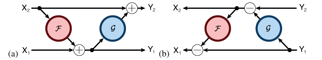
传统网络的块通常是不可逆的。RevNets 致力于构造输入与输出的双射,理论上实现可逆的无损传播。其可逆块分别有两个输入和输出,Forward 和 Backward 过程如下图 (a) (b) 所示。
公式表示
Forwardy1y2Backwardx2x1=x1+F(x2)=x2+G(y1)=y2−G(y1)=y1−F(x2)(1)
从而,可以使用 {y1,y2} 恢复 {x1,x2},以此类推。
可逆性条件
构造这样可逆块的充要条件是 块的雅可比矩阵具有单位行列式。 原文从梯度计算的角度给予解释
Because the model is invertible and its Jacobian has unit determinant, the log-likelihood and its gradients can be tractably computed. This architecture imposes some constraints on the functions the network can represent; for instance, it can only represent volume-preserving mappings.
比如,式 (1) 的雅可比行列式为
J=[1∂y1∂G⋅1∂x2∂F∂y1∂G∂x2∂F+1](2)
因此 ∣J∣=1,具有可逆性。
我们从还原输入的角度理解这一条件,它包含了如下必要条件
- 输入必须交叉,即 y2 的表达式含有 y1 或 x1,对 y1 同理。
- x1 和 x2 必须在两个表达式中独立出现过。
它们的作用分别是保证雅可比行列式中偏导数可消、提供常数。第 2 条不是很好理解,通过如下的例子解释
y1y2=x1+F(x2)=x1(3)
式 (3) 所描述的块就不是可逆的,因为 x2 在右式中只作为 F 的输入,而没有独立出现过。检查雅可比行列式
∣J∣=[11∂x2∂F0]=∂x2∂F(4)
不满足可逆性定义。
其他形式的可逆块
根据上一节介绍的可逆性条件,可以写出其他结构的可逆块。
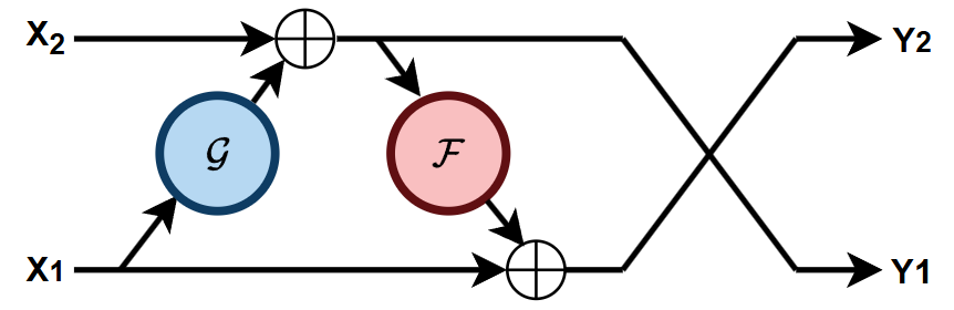
i. 含有两个函数 F,G 的
公式表示
y1y2=x2+G(x1)=x1+F(y1)(5)
反向先还原 x1,再还原 x2。可逆性验证
∣J∣=[∂x1∂G1+∂y1∂F∂x1∂G1∂y1∂F⋅1]=1(6)
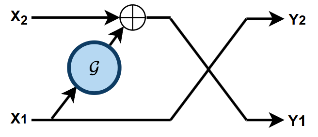
ii. 含有一个函数 G
公式表示
y1y2=x2+G(x1)=x1(7)
式 (7) 相当于式 (5) 取 F(⋅)=0,同样有 ∣J∣=1.
类似地,可以在式 (1) 取 G(⋅)=0,此时可逆块退化成 y1=x1+C,其实还是可逆的,虽然这样就没什么用了。
反向传播
可逆块的求导同样遵循链式法则
vi=j∈Child(i)∑(∂vi∂fj)⊤vj(8)
其中 Child(i) 表示 G 中节点 vi 的子节点 ,∂fj/∂vi 表示雅可比矩阵。
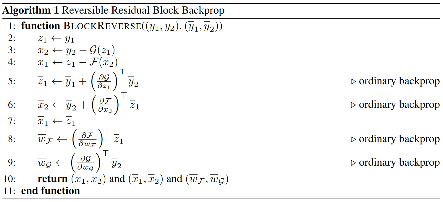
值得注意的是,可逆块的还原和求导对函数 F,G 不敏感。在还原过程中,我们不需要知道 F−1,G−1;在求导过程中,可以直接调用相应深度学习框架的自动求导函数对 F,G 求导。这个性质使得可以容易地将任意神经网络结构作为可逆块,只需在其前后添加可逆残差连接。
Note that Algorithm 1 is agnostic to the form of the residual functions F and G. The steps which use the Jacobians of these functions are implemented in terms of ordinary backprop, which can be achieved by calling automatic differentiation routines (e.g. tf.gradients or Theano.grad).
实际应用中,一般使用形如式 (7) 的含有一个函数的可逆块即足够,如 IDM (TPAMI 2025).
伪代码

Summary
这个可逆块还是受限的,比如输入输出必须形状相同。一些其他工作引入了更灵活的可逆变换 (如 exp 等),使其更加完善。
References
- 可逆神经网络(Invertible Neural Networks)详细解析:让神经网络更加轻量化-CSDN博客
- A. N. Gomez, M. Ren, R. Urtasun, and R. B. Grosse, “The Reversible Residual Network: Backpropagation Without Storing Activations,” in Advances in Neural Information Processing Systems, Curran Associates, Inc., 2017.